Voronoi Diagrams on a Spherical Surface

class voronoi_utility.Voronoi_Sphere_Surface(points, sphere_radius=None, sphere_center_origin_offset_vector=None)

Voronoi diagrams on the surface of a sphere.

Parameters:

points : array, shape (npoints, 3)

Coordinates of points used to construct a Voronoi diagram on the surface of a sphere.

sphere_radius : float

Radius of the sphere (providing radius is more accurate than forcing an estimate). Default: None (force estimation).

sphere_center_origin_offset_vector : array, shape (3,)

A 1D numpy array that can be subtracted from the generators (original data points) to translate the center of the sphere back to the origin. Default: None assumes already centered at origin.

Notes

The spherical Voronoi diagram algorithm proceeds as follows. The Convex Hull of the input points (generators) is calculated, and is equivalent to their Delaunay triangulation on the surface of the sphere [Caroli]. A 3D Delaunay tetrahedralization is obtained by including the origin of the coordinate system as the fourth vertex of each simplex of the Convex Hull. The circumcenters of all tetrahedra in the system are calculated and projected to the surface of the sphere, producing the Voronoi vertices. The Delaunay tetrahedralization neighbour information is then used to order the Voronoi region vertices around each generator. The latter approach is substantially less sensitive to floating point issues than angle-based methods of Voronoi region vertex sorting.

The surface area of spherical polygons is calculated by decomposing them into triangles and using L’Huilier’s Theorem to calculate the spherical excess of each triangle [Weisstein]. The sum of the spherical excesses is multiplied by the square of the sphere radius to obtain the surface area of the spherical polygon. For nearly-degenerate spherical polygons an area of approximately 0 is returned by default, rather than attempting the unstable calculation.

Empirical assessment of spherical Voronoi algorithm performance suggests quadratic time complexity (loglinear is optimal, but algorithms are more challenging to implement). The reconstitution of the surface area of the sphere, measured as the sum of the surface areas of all Voronoi regions, is closest to 100 % for larger (>> 10) numbers of generators.

References

[Caroli]

(1, 2) Caroli et al. Robust and Efficient Delaunay triangulations of points on or close to a sphere. Research Report RR-7004, 2009.

[Weisstein]

(1, 2) “L’Huilier’s Theorem.” From MathWorld–A Wolfram Web Resource. http://mathworld.wolfram.com/LHuiliersTheorem.html

Examples

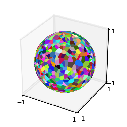
Produce a Voronoi diagram for a pseudo-random set of points on the unit sphere:

>>> import matplotlib
>>> import matplotlib.pyplot as plt
>>> import matplotlib.colors as colors
>>> from mpl_toolkits.mplot3d import Axes3D
>>> from mpl_toolkits.mplot3d.art3d import Poly3DCollection
>>> import numpy as np
>>> import scipy as sp
>>> import voronoi_utility
>>> #pin down the pseudo random number generator (prng) object to avoid certain pathological generator sets
>>> prng = np.random.RandomState(117) #otherwise, would need to filter the random data to ensure Voronoi diagram is possible
>>> #produce 1000 random points on the unit sphere using the above seed
>>> random_coordinate_array = voronoi_utility.generate_random_array_spherical_generators(1000,1.0,prng)
>>> #produce the Voronoi diagram data
>>> voronoi_instance = voronoi_utility.Voronoi_Sphere_Surface(random_coordinate_array,1.0)
>>> dictionary_voronoi_polygon_vertices = voronoi_instance.voronoi_region_vertices_spherical_surface()
>>> #plot the Voronoi diagram
>>> fig = plt.figure()
>>> fig.set_size_inches(2,2)
>>> ax = fig.add_subplot(111, projection='3d')
>>> for generator_index, voronoi_region in dictionary_voronoi_polygon_vertices.iteritems():
...    random_color = colors.rgb2hex(sp.rand(3))
...    #fill in the Voronoi region (polygon) that contains the generator:
...    polygon = Poly3DCollection([voronoi_region],alpha=1.0)
...    polygon.set_color(random_color)
...    ax.add_collection3d(polygon)
>>> ax.set_xlim(-1,1);ax.set_ylim(-1,1);ax.set_zlim(-1,1);
(-1, 1)
(-1, 1)
(-1, 1)
>>> ax.set_xticks([-1,1]);ax.set_yticks([-1,1]);ax.set_zticks([-1,1]); 
[<matplotlib.axis.XTick object at 0x...>, <matplotlib.axis.XTick object at 0x...>]
[<matplotlib.axis.XTick object at 0x...>, <matplotlib.axis.XTick object at 0x...>]
[<matplotlib.axis.XTick object at 0x...>, <matplotlib.axis.XTick object at 0x...>]
>>> plt.tick_params(axis='both', which='major', labelsize=6)

Now, calculate the surface areas of the Voronoi region polygons and verify that the reconstituted surface area is sensible:

>>> import math
>>> dictionary_voronoi_polygon_surface_areas = voronoi_instance.voronoi_region_surface_areas_spherical_surface()
>>> theoretical_surface_area_unit_sphere = 4 * math.pi
>>> reconstituted_surface_area_Voronoi_regions = sum(dictionary_voronoi_polygon_surface_areas.itervalues())
>>> percent_area_recovery = round((reconstituted_surface_area_Voronoi_regions / theoretical_surface_area_unit_sphere) * 100., 5)
>>> print percent_area_recovery
99.91979

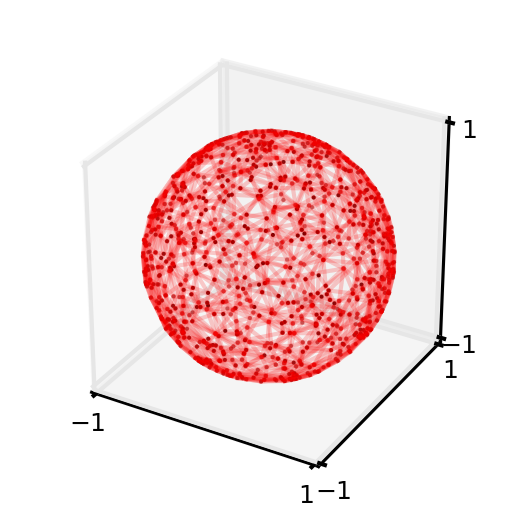
For completeness, produce the Delaunay triangulation on the surface of the unit sphere for the same data set:

>>> Delaunay_triangles = voronoi_instance.delaunay_triangulation_spherical_surface()
>>> fig2 = plt.figure()
>>> fig2.set_size_inches(2,2)
>>> ax = fig2.add_subplot(111, projection='3d')
>>> for triangle_coordinate_array in Delaunay_triangles:
...     m = ax.plot(triangle_coordinate_array[...,0],triangle_coordinate_array[...,1],triangle_coordinate_array[...,2],c='r',alpha=0.1)
...     connecting_array = np.delete(triangle_coordinate_array,1,0)
...     n = ax.plot(connecting_array[...,0],connecting_array[...,1],connecting_array[...,2],c='r',alpha=0.1)
>>> o = ax.scatter(random_coordinate_array[...,0],random_coordinate_array[...,1],random_coordinate_array[...,2],c='k',lw=0,s=0.9)
>>> ax.set_xlim(-1,1);ax.set_ylim(-1,1);ax.set_zlim(-1,1);
(-1, 1)
(-1, 1)
(-1, 1)
>>> ax.set_xticks([-1,1]);ax.set_yticks([-1,1]);ax.set_zticks([-1,1]); 
[<matplotlib.axis.XTick object at 0x...>, <matplotlib.axis.XTick object at 0x...>]
[<matplotlib.axis.XTick object at 0x...>, <matplotlib.axis.XTick object at 0x...>]
[<matplotlib.axis.XTick object at 0x...>, <matplotlib.axis.XTick object at 0x...>]
>>> plt.tick_params(axis='both', which='major', labelsize=6)

Methods

delaunay_triangulation_spherical_surface()	Delaunay tessellation of the points on the surface of the sphere.
voronoi_region_surface_areas_spherical_surface()	Returns a dictionary with the estimated surface areas of the Voronoi region polygons corresponding to each generator (original data point) index.
voronoi_region_vertices_spherical_surface()	Returns a dictionary with the sorted (non-intersecting) polygon vertices for the Voronoi regions associated with each generator (original data point) index.

delaunay_triangulation_spherical_surface()

Delaunay tessellation of the points on the surface of the sphere. This is simply the 3D convex hull of the points. Returns a shape (N,3,3) array of points representing the vertices of the Delaunay triangulation on the sphere (i.e., N three-dimensional triangle vertex arrays).

voronoi_region_surface_areas_spherical_surface()

Returns a dictionary with the estimated surface areas of the Voronoi region polygons corresponding to each generator (original data point) index. An example dictionary entry: {generator_index : surface_area, ...}.

voronoi_region_vertices_spherical_surface()

Returns a dictionary with the sorted (non-intersecting) polygon vertices for the Voronoi regions associated with each generator (original data point) index. A dictionary entry would be structured as follows: {generator_index : array_polygon_vertices, ...}.